dracoblue.net

This post documents Week 2 of the TopicWatchdog project.
Last week we successfully extracted topics and claims from German political short videos and persisted them in BigQuery.
However, topics often appeared under slightly different names — making aggregation unreliable.

This week we explore embeddings + clustering:

• Generate embeddings of canonical topics and claims with BigQuery ML.
• Train a KMeans model on those embeddings to group semantically similar entries.
• Assign clusters back to each topic/claim.
• Inspect first results in Looker Studio and reflect on limitations.

Table of Contents

1. Why embeddings? (motivation for moving beyond string matching)
2. Generating embeddings with BigQuery ML (SQL + table design)
3. Training KMeans for clustering (model creation + options)
4. Assigning clusters to topics (ML.PREDICT + join back to topics)
5. Generating Human-Readable Cluster Labels
6. Early results & charts (Looker Studio examples)
7. Limitations & Next Steps

1) Why Embeddings?

In Kickoff (Week 1): Extracting Topics & Claims from German Politics Videos we saw that the same political topic appeared under slightly different names — for example "Migration stoppen" vs. "Grenzschutz verschärfen".
A simple GROUP BY canonical could not merge such near-synonyms reliably.

To address this, we moved towards semantic embeddings:
- Every topic string (the canonical field from Week-1 extraction) is transformed into a vector representation using ML.GENERATE_EMBEDDING.
- Similar topics have embeddings close to each other in vector space.
- Once embedded, we can apply clustering algorithms (like KMeans) directly inside BigQuery ML, without leaving the warehouse.

This step turns our raw text into structured numeric data that can be clustered and compared across time.

2) Generating Embeddings with BigQuery ML

The extracted topics live in the table topicwatchdog.fact_topics, where each row has a canonical form.
To prepare them for clustering, we generate embeddings using the Vertex-AI text embedding model connected to BigQuery.

First of all we need to have a proper connection created via Create Cloud resource connections. I generated it in the eu and called it vertex-ai-eu-conn.

Afterwards I use this connection and create a model to have the proper embedding model available:

CREATE OR REPLACE MODEL `topicwatchdog.text_embedding`
REMOTE WITH CONNECTION `eu.vertex-ai-eu-conn`
OPTIONS(ENDPOINT = 'text-multilingual-embedding-002');

I use text-multilingual-embedding-002 since it works great for multi language stuff and we do have german texts.

We store results in a separate table topicwatchdog.fact_topic_embeddings to keep things reproducible. First of all we create the table:

CREATE TABLE IF NOT EXISTS `topicwatchdog.fact_topic_embeddings` (
  video_youtube_id STRING NOT NULL,
  topic             STRING,
  emb              ARRAY<FLOAT64>,
  topic_timestamp  DATE
)
PARTITION BY topic_timestamp
CLUSTER BY video_youtube_id;

Since I am a big fan of updating embeddings only if new fact_topics are generated which we don't know yet: we JOIN them like this and check for NULL and generate them only in this case.

INSERT INTO `topicwatchdog.fact_topic_embeddings` (
  video_youtube_id, topic, emb, topic_timestamp
)
SELECT
  ge.video_youtube_id,
  ge.content AS topic,
  ge.ml_generate_embedding_result AS emb, 
  DATE(ge.topic_timestamp) AS topic_timestamp
FROM ML.GENERATE_EMBEDDING(
  MODEL `topicwatchdog.text_embedding`,   
  (
    SELECT
      ft.video_youtube_id,
      ft.topic AS content,
      ft.topic_timestamp
    FROM `topicwatchdog.fact_topics` ft
    LEFT JOIN `topicwatchdog.fact_topic_embeddings` fte ON (fte.video_youtube_id = ft.video_youtube_id AND fte.topic = ft.topic)
    WHERE fte.video_youtube_id IS NULL
  ),
  STRUCT(TRUE AS flatten_json_output)
) AS ge

This will have one embedding per (video_youtube_id, topic) pair. Later, we can also test embeddings per ressort or parent for higher-level clustering.

3) Training KMeans for Clustering

With embeddings available, we can now train a clustering model directly in BigQuery ML.
For Week-2 I chose KMeans, since it is well supported in BigQuery and fast to experiment with.

The following SQL creates a model with 20 clusters:

CREATE OR REPLACE MODEL `topicwatchdog.kmeans_topics`
OPTIONS(
  MODEL_TYPE = 'kmeans',
  NUM_CLUSTERS = 20,
  STANDARDIZE_FEATURES = TRUE
) AS
SELECT
  emb
FROM `topicwatchdog.fact_topic_embeddings`;

Design choices:

• NUM_CLUSTERS=20 was an initial guess. In practice, you can tune this parameter by computing the silhouette score or trying values via a parameter sweep.
• STANDARDIZE_FEATURES=TRUE ensures embeddings are normalized before clustering.
• Training stays inside BigQuery, so no external pipelines or exports are required.

The output is a reusable model object topicwatchdog.kmeans_topics which we can now use for predictions.

4) Assigning Clusters to Topics

To make the clusters usable for analysis, we run ML.PREDICT and join the results back to the original topics.

CREATE OR REPLACE TABLE `topicwatchdog.fact_topic_clusters` AS
SELECT
  t.video_youtube_id,
  t.topic,
  p.centroid_id AS cluster_id,
  p.nearest_centroids_distance[OFFSET(0)].distance AS cluster_distance
FROM ML.PREDICT(MODEL `topicwatchdog.kmeans_topics`,
  (
    SELECT
      emb,
      video_youtube_id,
      topic,
    FROM `topicwatchdog.fact_topic_embeddings`
  )
) p
JOIN `topicwatchdog.fact_topic_embeddings` t
USING(video_youtube_id, topic);

What this does:

• Each topic is assigned to its nearest centroid.
• We keep the distance field to later evaluate cluster cohesion (smaller = better fit).
• Results are stored in topicwatchdog.fact_topic_clusters, which can be aggregated in Looker Studio or further processed (e.g. by averaging cluster labels).

This gives us a practical way to see which different canonical topics (like “Migration stoppen” vs. Grenzschutz) fall into the same semantic cluster.

5) Generating Human-Readable Cluster Labels

Cluster IDs are just numbers (0–19 in our case).
To make the results interpretable in dashboards, we create a mapping table fact_topic_clusters_map with human-readable names.

The workflow:

1. For each cluster, sample ~20 representative topics.
   
2. Prompt an LLM to propose a short, neutral label that summarizes the cluster.
   
3. Store the result in a mapping table.

Example SQL to collect 20 samples per cluster:

  CREATE TEMP TABLE _cluster_examples AS
  SELECT
    cluster_id,
    ARRAY_AGG(topic ORDER BY topic LIMIT 20) AS examples,
    COUNT(*) AS n
  FROM `topicwatchdog.fact_topic_clusters`
  GROUP BY cluster_id
  HAVING COUNT(*) > 5;

We can then feed _cluster_examples into an LLM (Vertex AI Text model) with a structured prompt:

CREATE TEMP TABLE _prompts_topics AS
SELECT
cluster_id,
(
    'Du bist politischer Analyst. Vergib einen prägnanten, verständlichen ' ||
    'Titel (max. 60 Zeichen) für diesen **Themen**-Cluster. ' ||
    'Regeln: deutsch, neutral, keine neuen Themen/Namen erfinden, ' ||
    'nur EIN kurzer Titel. Antworte strikt Text ohne Markdown oder json. ' ||
    '\n\nBeispiele (Original-Canonicals):\n' ||
    STRING_AGG('- ' || ex, '\n')
) AS prompt
FROM _cluster_examples, UNNEST(examples) AS ex
GROUP BY cluster_id;

Now we have _prompt_topics temp table full of prompts. We want to use gemini-2.5-flash-lite the flash lite version of gemini to generate these cluster labels, so we need a remote model created for this:

CREATE OR REPLACE MODEL `gemini-2.5-flash-lite`
  REMOTE WITH CONNECTION `eu.vertex-ai-eu-conn'`
  OPTIONS (ENDPOINT = 'topicwatchdog.gemini_remote')

Finally, we use the Gemini remote model to generate labels and persist them into fact_topic_clusters_map:

CREATE OR REPLACE TABLE `topicwatchdog.fact_topic_clusters_map` AS
SELECT
  cluster_id,
  ml_generate_text_llm_result AS cluster_label
FROM ML.GENERATE_TEXT(
  MODEL `topicwatchdog.gemini_remote`,
  TABLE _prompts_topics,
  STRUCT(
    TRUE AS flatten_json_output,
    0.2 AS temperature,
    256 AS max_output_tokens
  )
) AS gen;

Result: We now have a persistent table fact_topic_clusters_map mapping numeric cluster IDs → stable human-readable names like:

| cluster_id  | cluster_label                |
| ----------- | ---------------------------- |
| 1           | Arbeit und soziale Sicherung |
| 2           | Gesundheitssystem            |
| …           | …                            |

This makes Looker Studio dashboards far easier to interpret.

6) Early Results & Charts

With clusters assigned, we can finally see how topics group together in practice.

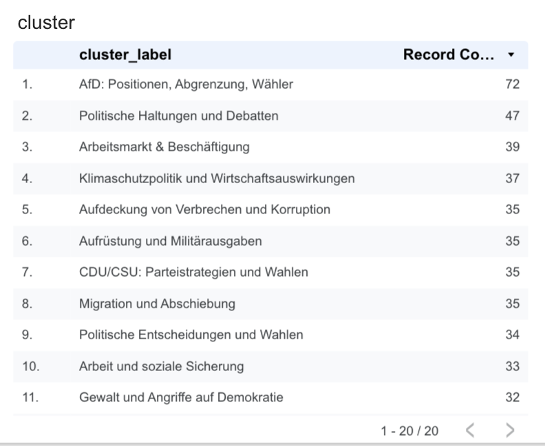
In Looker Studio I built two quick views:

1. Cluster Distribution
   A pie chart of cluster_id counts shows how many topics fall into each group.
   This already reveals that some clusters are dominant (e.g. “Migration & Grenzschutz”), while others capture niche topics.

Figure: First Looker Studio visualization of clusters.

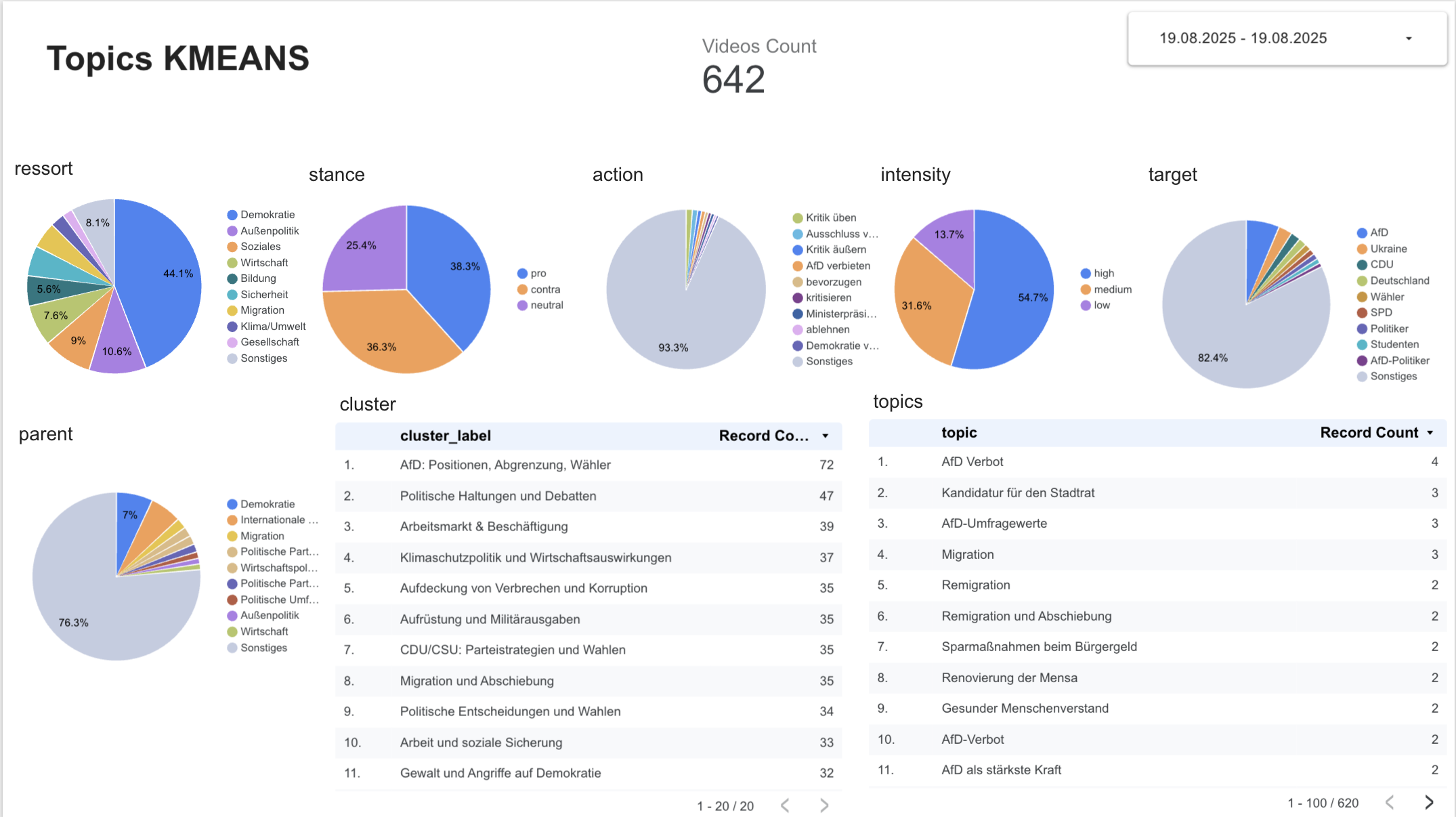
1. Topic Table by Cluster
   A table listing cluster_id, topic, and distance.
   This view helps check if the canonical variants we hoped to merge actually appear together.
   For example:
   
   • “Migration stoppen”
     
   • “Grenzschutz verschärfen”
     all ended up in the same cluster.

Figure: First Looker Studio visualization of clustered topics.

While not perfect, these early charts show that embedding + clustering works much better than the plain string grouping from Week-1.

7) Limitations & Next Steps

While the embedding + clustering approach shows clear improvements, there are still important caveats:

• Cluster count is arbitrary
  KMeans requires NUM_CLUSTERS. My choice of 20 was heuristic. Different values change the grouping significantly. A next step is to run parameter sweeps and evaluate metrics like silhouette score.

• Synonyms vs. nuance
  Some clusters still mix semantically close but contextually different topics (e.g. “EU-Erweiterung” vs. “EU-Austritt”). Canonicalization + human review remain necessary.

• Drift over time
  Topics evolve. A cluster trained on August data may not perfectly match clusters from September. I need to monitor drift and possibly retrain models regularly.

• Claims excluded
  In Week-2, clustering was limited to topics. Claims will follow once the topic pipeline is stable.

Next steps:

• Evaluate optimal cluster count using ML.EVALUATE.
  
• Experiment with hierarchical clustering or HDBSCAN via BERTopic outside BigQuery.
  
• Build a lightweight human-in-the-loop labeling UI in PayloadCMS, so clusters can be reviewed and renamed.
  
• Use clusters as stable Topic IDs for longitudinal analysis.

This closes Week-2: Topics now live not just as strings, but as structured clusters in BigQuery ML.